Project - Fabian Thüring (12-936-241)

Project Idea

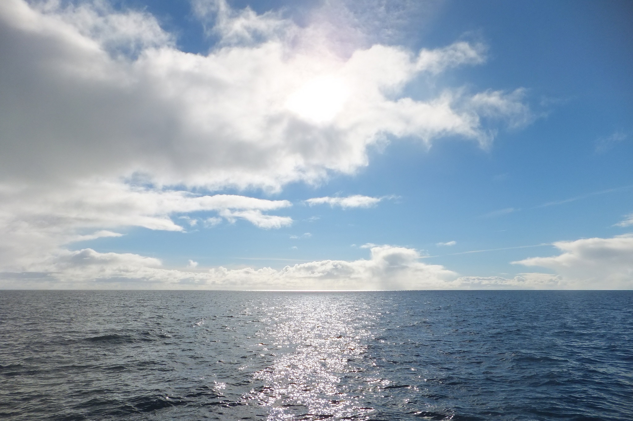
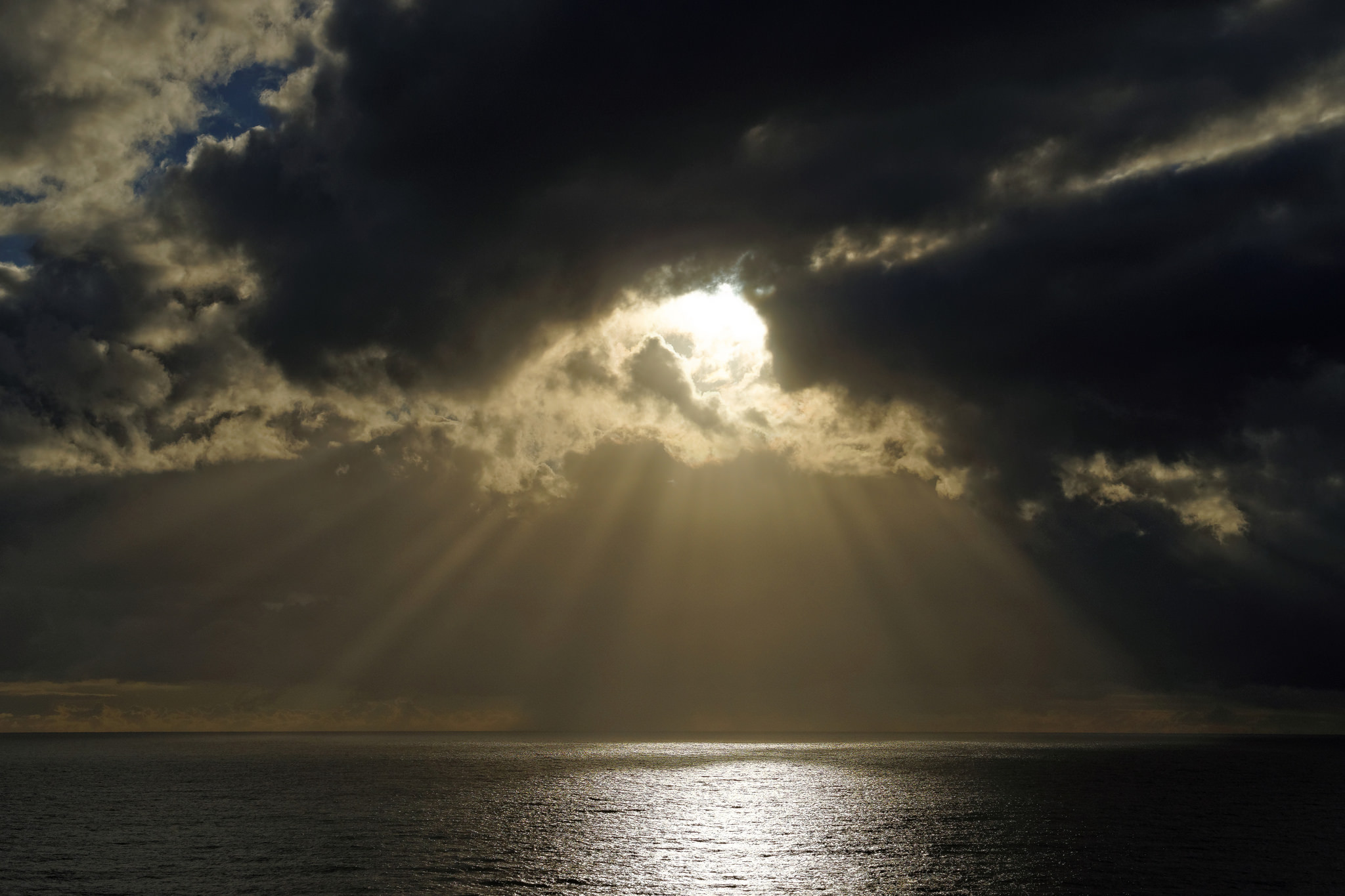
Water, among fire, earth and air is one of the classical elements and the key to life as we encounter it on this planet. This project will depict a scene which is the embodiment of water, the ocean. As our atmosphere usually isn't homogenous, we have small cloud formations in the lower troposphere which can beautifully interact with the sun light and create this marvelously looking scenery as shown in the images below.

Refrence image

Implemented features

Depth of Field (5 Points)

Cameras in the real world have lens systems which focus the light through a finite-sized aperture onto the film plane, as opposed to pinhole cameras which have infinitesimal aperture. Consequently, a point might be projected onto an area (circle of confusion) which results in a blurred image. This effect is called depth-of-field. In this section I've added support for depth-of-field by extending the perspective camera (Perspective::sampleRay). Two new parameters have been introduced:

• lensRadius: Control the radius of the lens.
• focalDistance: The distance to the focal plane (where radius of circle of confusion is zero)

The general implementation idea is the following: First, we sample a point on the lens by sampling a uniform disk and scale the sample with the radius of the lens. Secondly, we determine the proper direction of the new ray and apply all transformations to world space.

Relevant files:

• perspective.cpp

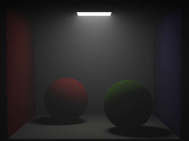
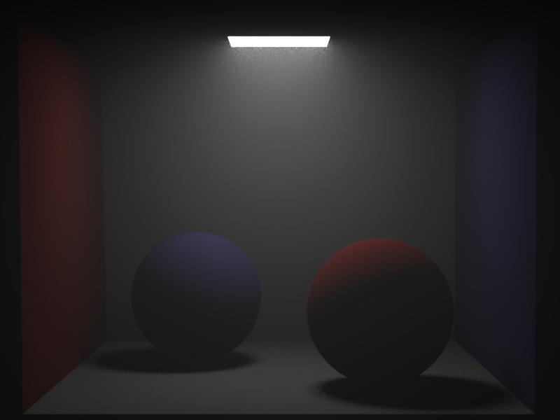
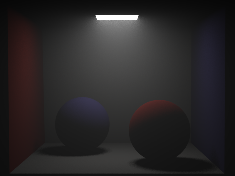
Cornell box scene

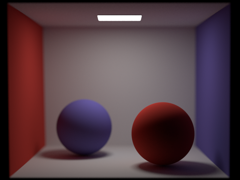
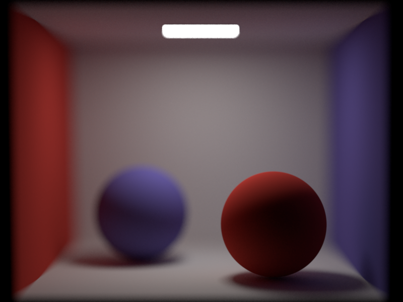
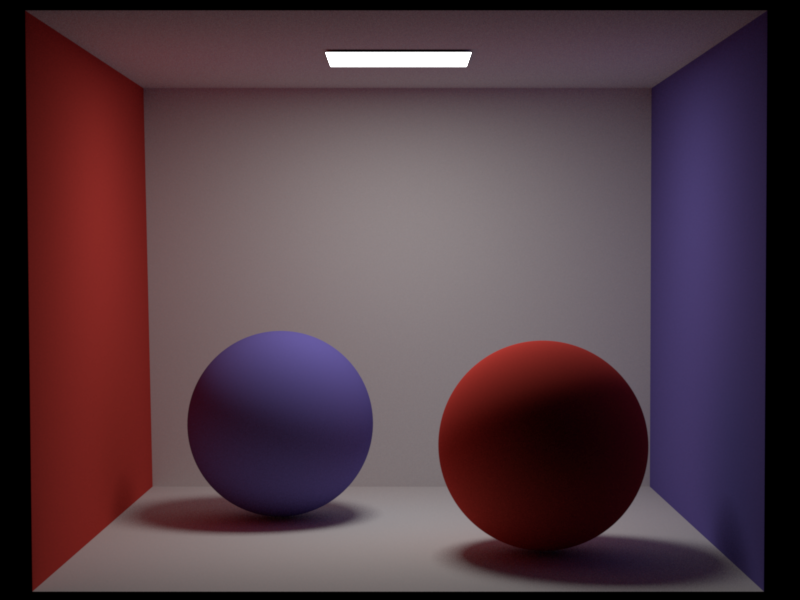
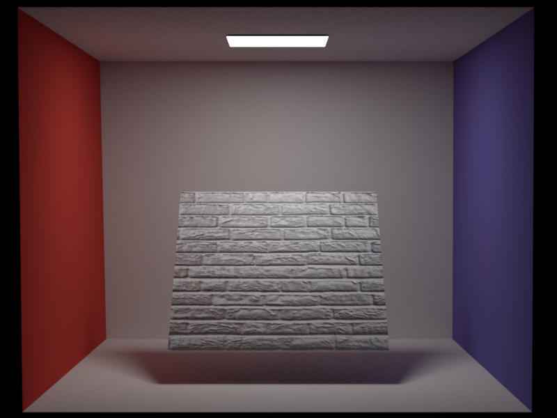
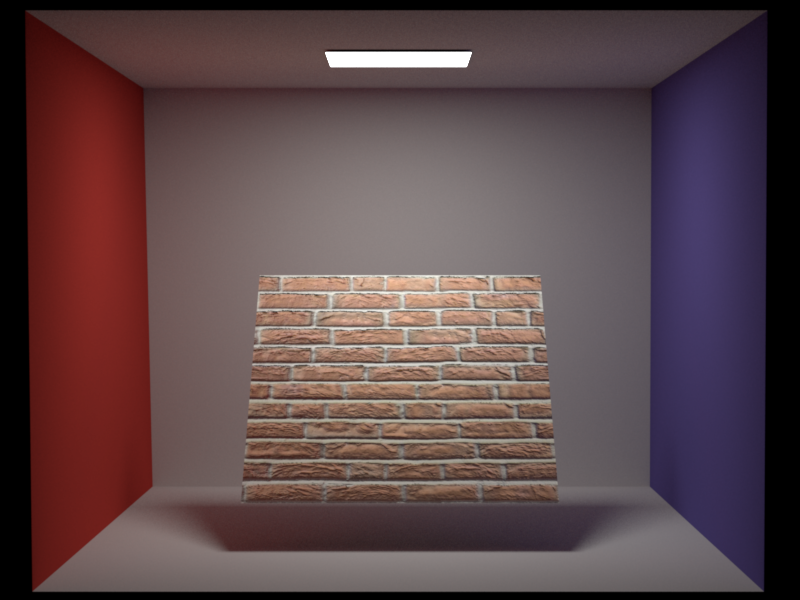
The following Cornell box scene was rendered with the MIS path tracing integrator using 512 samples per pixel. The images below show a focal distance matching the front spheres depth with a lens radius of 0.1 and 0.3. The image to the right clearly shows the effect of a larger lens radius wich results in an increase of blurriness with increasing distance to the focal plane.

.

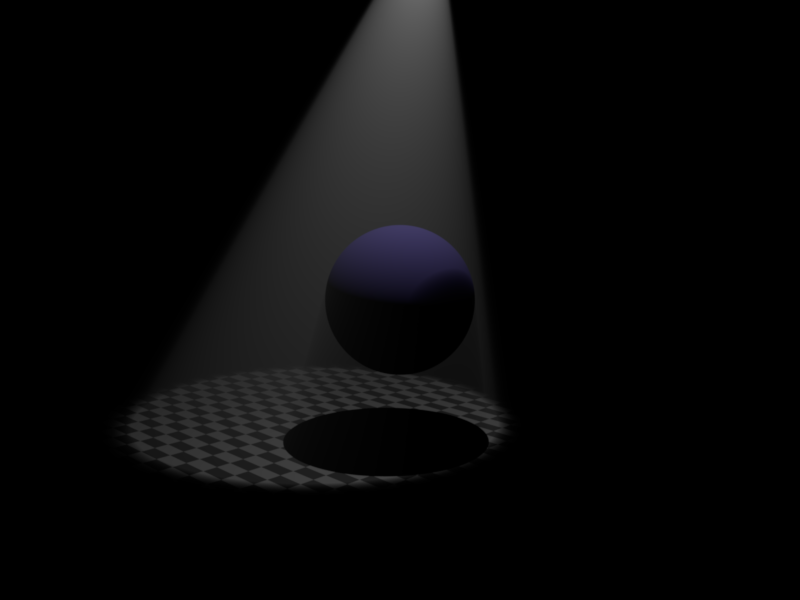
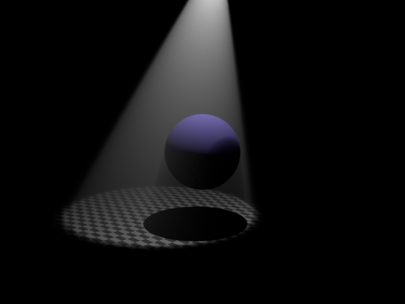
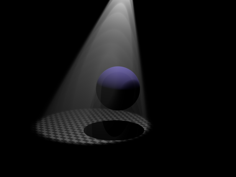
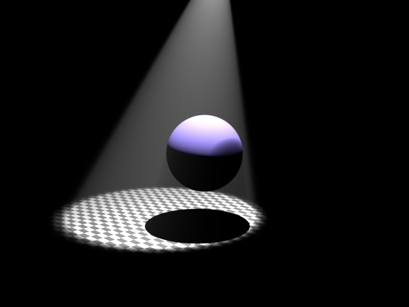
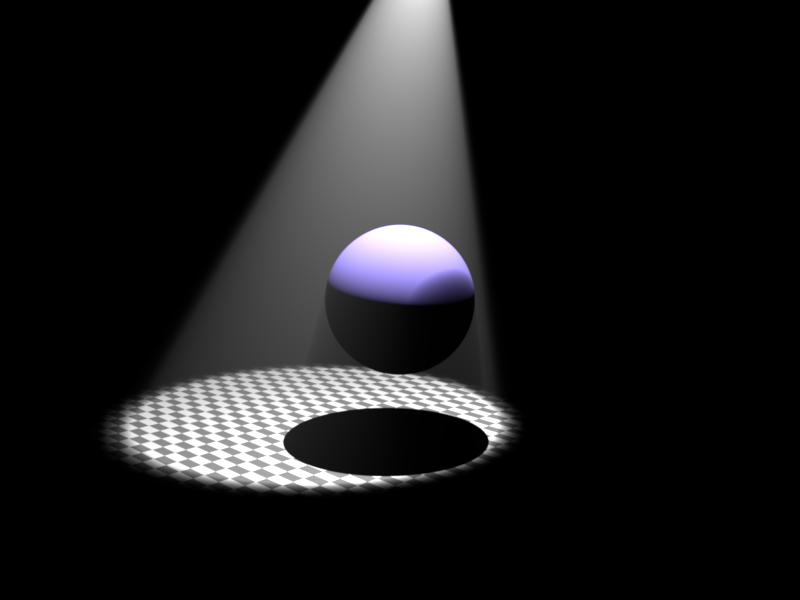
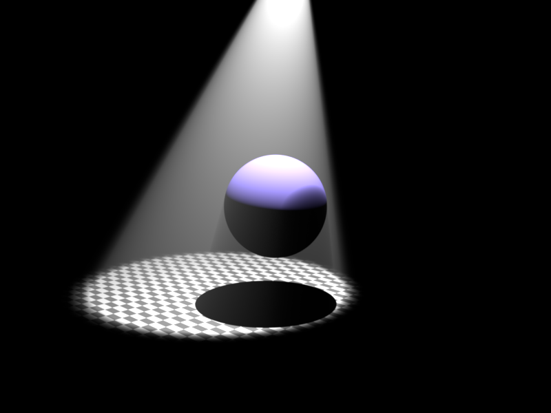
Spot light emitter (5 Points)

Spot lights are a variation of point lights with emitting light in a cone of directions from their position. In addition to position and power the spot light has a new parameter direction \(\vec{d}_s\). The cone is specified by two additional parameters width and falloff. The width angle \(\theta_{w}\), in degrees, specifies the extend of the cone while the falloff angle \(\theta_{f}\) is responsible for smoothing out the transition from full illumination, inside the cone, to none, outside the cone. Therefore, it must always hold \( 0 \leq \theta_{f} \leq \theta_{w} \leq 180\).

Given a direction to the light source \(\vec{w}_i\) and the direction of emission of the spot light \(\vec{d}_s\), we can compute the angle between the two vectors: \(\theta = \cos^{-1}(-\vec{w}_i\cdot\vec{d}_s)\) and the occlusion (which will be multiplied with the radiance) can be calculated like this:

\( occlusion(\theta) = \begin{cases} 0, & \theta \geq \theta_w \\ \left(\frac{\cos\theta - \cos\theta_w}{\cos\theta_f - \cos\theta_w}\right)^4,& \theta_f \leq \theta \leq \theta_w \\ 1, & \text{otherwise} \end{cases} \)

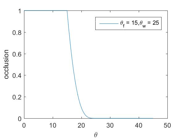
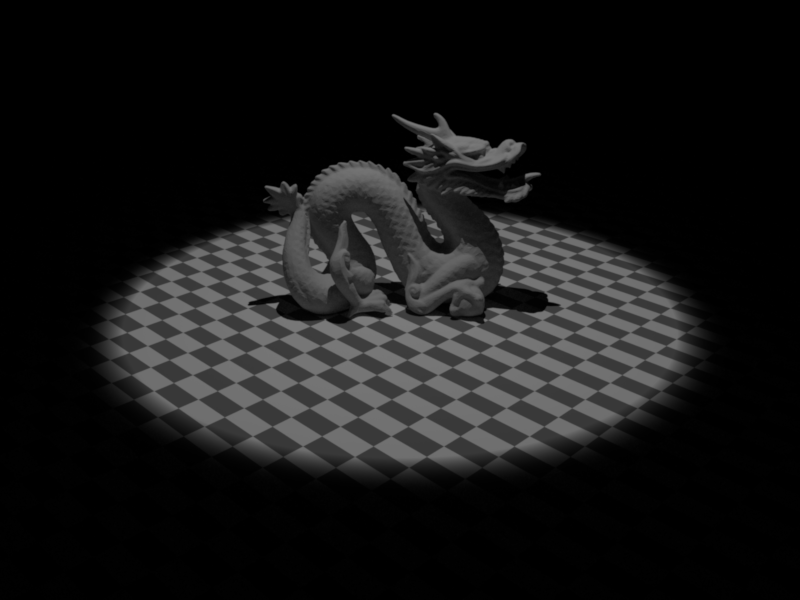
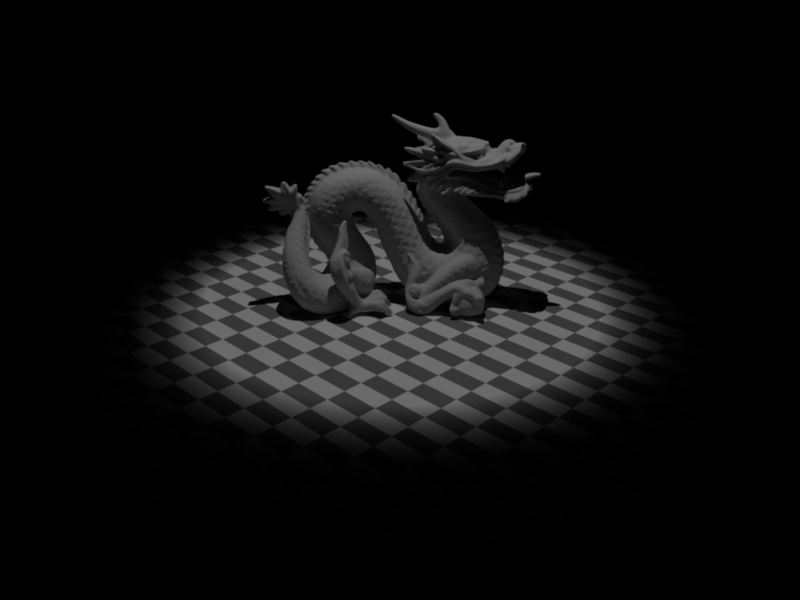
In the first case we are outside the light cone, hence the radiance must be 0. In the second case we are in the falloff area which is represented by a fourth order polynomial. The images below showcase the effect of the falloff with the second image having a much bigger falloff area than the first one.

Relevant files:

• spotlight.cpp

Cluster version of nori (5 Points)

Nori is tightly coupled to nanogui, an OpenGL based graphical user interface. While this comes in very handy when debugging the rendering process, it is unsuitable for rendering on server based clusters like EULER. In order to circumvent this problem I've added a new executable nori-cluster. This allows rendering without any X-Server running and hence can be executed on EULER. The new files cluster.h and cluster.cpp facilitate this task, while the updated CMake file ensures a correct building procedure. Below is an output of ldd(1) which shows the reduced object dependencies of nori-cluster compared to nori.

In addition to make the rendering process less error prone, rendering checkpoints have been added which periodically, based on user input parameters, save the current image. Aswell as command-line arguments to set the number of threads being used by TBB to prevent nori from hijacking the entire system.

Relevant files:

• cluster.h
• cluster.cpp
• main_cluster.cpp
• CMakeLists.txt

>$ ldd ./nori-cluster
>$ linux-vdso.so.1 =>  (0x00007fff27304000)
>$ libpthread.so.0 => /lib/x86_64-linux-gnu/libpthread.so.0 (0x00007fa08a0d7000)
>$ libz.so.1 => /lib/x86_64-linux-gnu/libz.so.1 (0x00007fa089ebe000)
>$ libdl.so.2 => /lib/x86_64-linux-gnu/libdl.so.2 (0x00007fa089cba000)
>$ libstdc++.so.6 => /usr/lib/x86_64-linux-gnu/libstdc++.so.6 (0x00007fa0899ad000)
>$ libm.so.6 => /lib/x86_64-linux-gnu/libm.so.6 (0x00007fa0896a7000)
>$ libgcc_s.so.1 => /lib/x86_64-linux-gnu/libgcc_s.so.1 (0x00007fa089490000)
>$ libc.so.6 => /lib/x86_64-linux-gnu/libc.so.6 (0x00007fa0890cb000)

>$ ldd ./nori
>$ linux-vdso.so.1 =>  (0x00007ffc635fd000)
>$ libGL.so.1 => /usr/lib/nvidia-352/libGL.so.1 (0x00007fa7d0ef3000)
>$ libXxf86vm.so.1 => /usr/lib/x86_64-linux-gnu/libXxf86vm.so.1 (0x00007fa7d0ced000)
>$ libXrandr.so.2 => /usr/lib/x86_64-linux-gnu/libXrandr.so.2 (0x00007fa7d0ae3000)
>$ libXinerama.so.1 => /usr/lib/x86_64-linux-gnu/libXinerama.so.1 (0x00007fa7d08e0000)
>$ libXcursor.so.1 => /usr/lib/x86_64-linux-gnu/libXcursor.so.1 (0x00007fa7d06d6000)
>$ libXi.so.6 => /usr/lib/x86_64-linux-gnu/libXi.so.6 (0x00007fa7d04c6000)
>$ libX11.so.6 => /usr/lib/x86_64-linux-gnu/libX11.so.6 (0x00007fa7d0191000)
>$ libpthread.so.0 => /lib/x86_64-linux-gnu/libpthread.so.0 (0x00007fa7cff73000)
>$ libz.so.1 => /lib/x86_64-linux-gnu/libz.so.1 (0x00007fa7cfd5a000)
>$ libdl.so.2 => /lib/x86_64-linux-gnu/libdl.so.2 (0x00007fa7cfb56000)
>$ libstdc++.so.6 => /usr/lib/x86_64-linux-gnu/libstdc++.so.6 (0x00007fa7cf849000)
>$ libm.so.6 => /lib/x86_64-linux-gnu/libm.so.6 (0x00007fa7cf543000)
>$ libgcc_s.so.1 => /lib/x86_64-linux-gnu/libgcc_s.so.1 (0x00007fa7cf32c000)
>$ libc.so.6 => /lib/x86_64-linux-gnu/libc.so.6 (0x00007fa7cef67000)
>$ libnvidia-tls.so.352.63 => /usr/lib/nvidia-352/tls/libnvidia-tls.so.352.63 (0x00007fa7ced64000)
>$ libnvidia-glcore.so.352.63 => /usr/lib/nvidia-352/libnvidia-glcore.so.352.63 (0x00007fa7cc2d1000)
>$ libXext.so.6 => /usr/lib/x86_64-linux-gnu/libXext.so.6 (0x00007fa7cc0bf000)
>$ libXrender.so.1 => /usr/lib/x86_64-linux-gnu/libXrender.so.1 (0x00007fa7cbeb5000)
>$ libXfixes.so.3 => /usr/lib/x86_64-linux-gnu/libXfixes.so.3 (0x00007fa7cbcaf000)
>$ libxcb.so.1 => /usr/lib/x86_64-linux-gnu/libxcb.so.1 (0x00007fa7cba90000)
>$ /lib64/ld-linux-x86-64.so.2 (0x00007fa7d1223000)
>$ libXau.so.6 => /usr/lib/x86_64-linux-gnu/libXau.so.6 (0x00007fa7cb88c000)

Normal and texture mapping (10 Points)

In order to get more realism out of the scene I've implemented normal and texture mapping in nori. To load the png image into memory I made use of the excellent and lightweight lodePNG library. The main class for texture mapping is PngTexture which derives from Texture. The texture maps are associated with a BRDF (diffuse or microfacet) and the normal maps will be paired with a shape.

Relevant files:

• texture.h
• pngtexture.cpp
• sphere.cpp
• mesh.cpp

Texture mapping

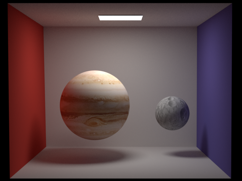
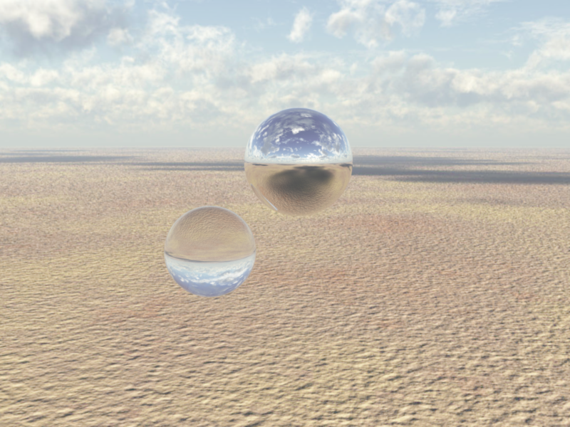
Given a pair of \((u,v)\) coordinates our task is to convert this into the pixel coordinates and return an albedo. If the \((u,v)\) coordinates are between \([0,1]\) the mapping is rather straight forward. However, if the coordinates lay in an arbitrary interval we have to apply some sort of transformation: I decided to implement the technique of replication. The first image below shows two texture mapped spheres (Jupiter and Mars) rendered with a 512 sample per pixel Path MIS integrator using a diffuse BRDF.

The following images show the replication of the texture (and corresponding normal map aswell). In the right image the \((u,v)\) coordinates lay in \([0,4]^2\) and hence the image is replicated 16 times where in the left we have the reference in \([0,1]^2\).

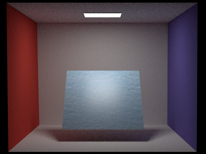
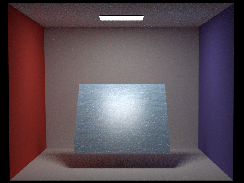
When using a microfacet BRDF one has to pay close attention to ensure energy conservation. In the exercise we did this by scaling the specular component with (1 - kd).maxCoeff() where kd is the albedo of the diffuse material. When using a texture as albedo we have to make sure that we adjust this scaling progressively. In the images below we can see the difference between being and being not energy conservant:

Normal mapping

The normal map works internally almost the same as a texture map with a subtle difference in how the map is going to be evaluated. Given a \((u,v)\) value we can calculate the pixel coordinate \((i,j)\) and retrieve the \((r,g,b)\) value of the map. Next we have to apply a linear transformation \([0,1] \rightarrow [-1,1]\). The final normal is calculated as:

\(\vec{n} = \left( \begin{array}{c} 2r - 1 \\ 2g - 1 \\ 2b - 1 \\ \end{array} \right)\)

The resulting normal will be re-normalized and transformed into to the shFrame.toWorld of the mesh or sphere when being called in setHitInformation.

Results

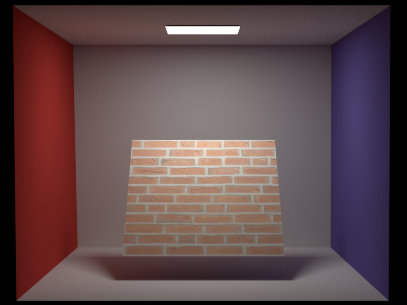
Below we can see a three-way comparison of normal and texture mapping. The image was rendered with the Path MIS integrator using 512 samples per pixel and a diffuse BRDF. We clearly observe that the application of normal and texture mapping yield a much nicer looking image than simple texture mapping.

Environment map emitter with importance sampling (15 Points)

Environment mapping is an efficient image-based rendering technique to approximate a reflective surrounding surface. In our case the environmentmap is a simple png or exr image, parametrized by longitude \(\theta\) and \(\phi\) latitude coordinates. The EnviromentMap class is treated as an Emitter and hence inherits from Emitter. Like any other Emitter it must provide a sampling method. A naive approach would be to simply sample a uniform sphere and convert the \((\theta,\phi)\) coordinates to the corresponding \((u,v)\) coordinates of the image. We shall use a more sophisticated approach presented by Matt Phar and Greg Humphreys [1] which is based on sampling the marginal and conditional probability density function independently.

Relevant files:

• environmentmap.cpp

Theory

Our goal is to draw samples from \(p(\theta,\phi) \propto L_{env}(\theta,\phi)\sin \theta\). The approach can be roughly split in 4 steps:

1. Create a scalar version \(f(\theta, \phi)\) of the image. This can be done by taking the luminance, maximum or the average of the RGB channels. All three options are supported in the implementation and can be controlled by the flag scalarize (all the image here use the luminance). In addition, we scale \(f\) with \(\sin\theta\).
2. Compute the marginal pdf \(p(\theta) = \int^{2\pi}_0 f(\theta, \phi) d\phi \rightarrow p_i = \sum^M_{j=0} f_{i,j}\) with \(f_{i,j}\) being the scalarized image of size \(N \times M\).
3. Compute conditional pdf \(p(\phi|\theta) = \frac{p(\theta,\phi)}{p(\theta)}\)
4. Draw samples \(\theta \propto p(\theta)\) and \(\phi = p(\phi|\theta)\).

Further details can be found in environmentmap.cpp

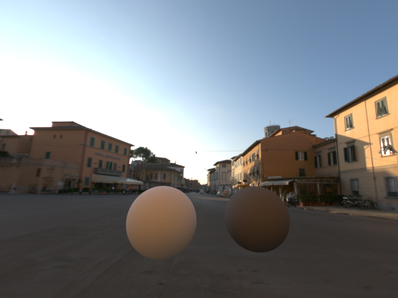
Results

The question remains does it work and is it worth it? The following two comparisons will outline the problem. In the first comparison one can not spot any difference between the importance sampled image and the simple sampled one at all. However, in the second comparison the importance sampled image has way less noise than the simple sampled one. We can conclude that if the environment map has a few very bright spots (like the ceiling lights in the chapel) and is mostly dark elsewhere, importance sampling can greatly improve the quality of the rendered image. On the other hand, if the image has a more continuous luminance, importance sampling does not noticeably improve the quality.

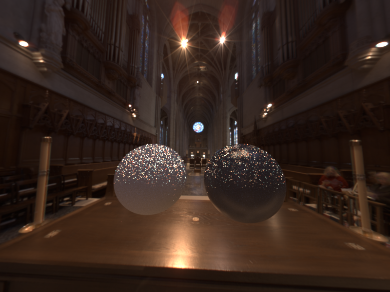
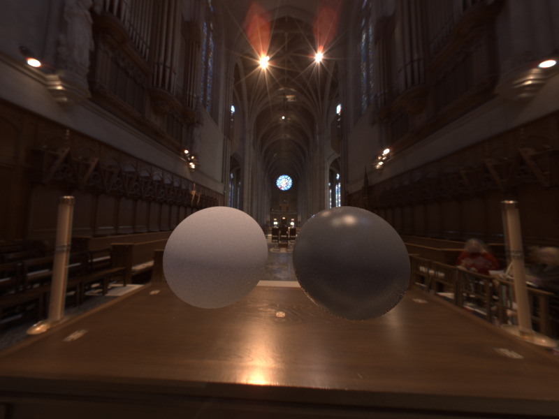
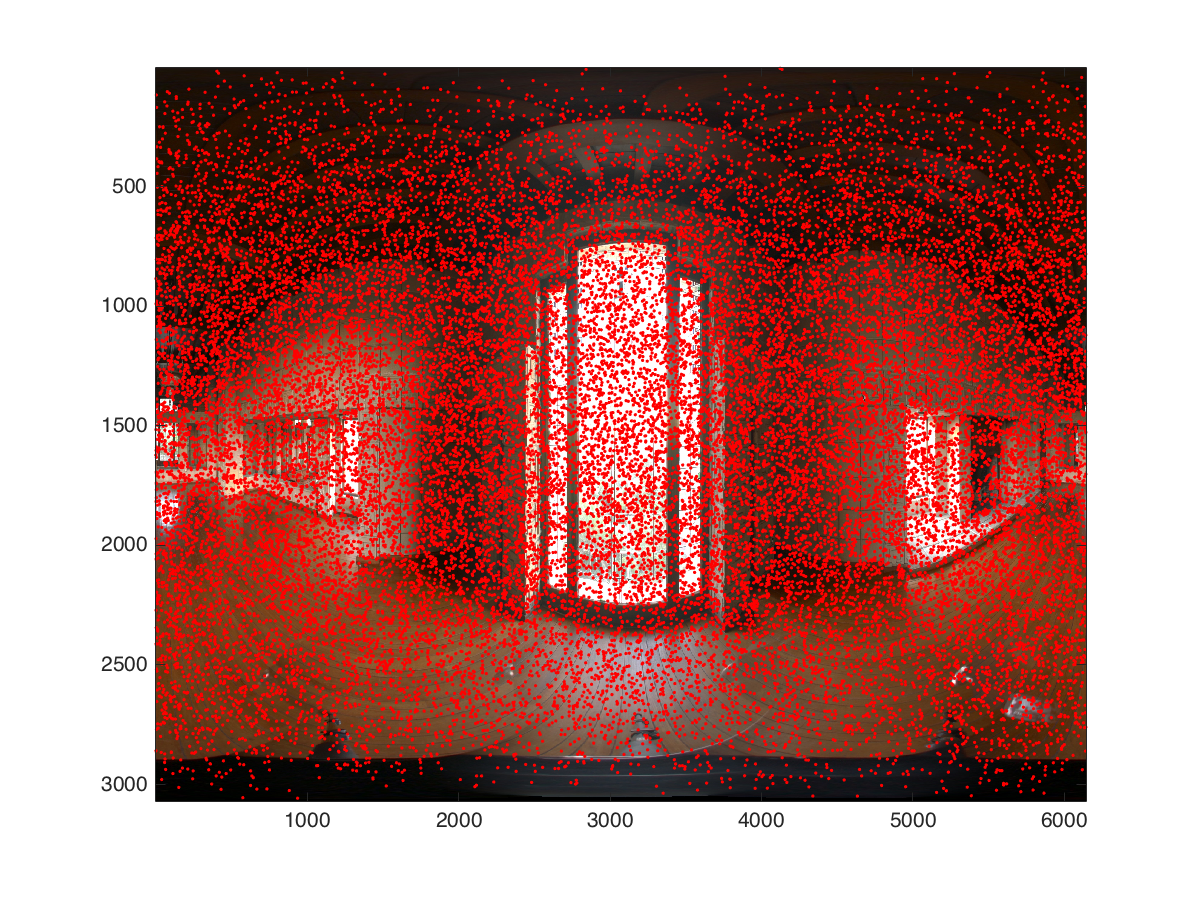
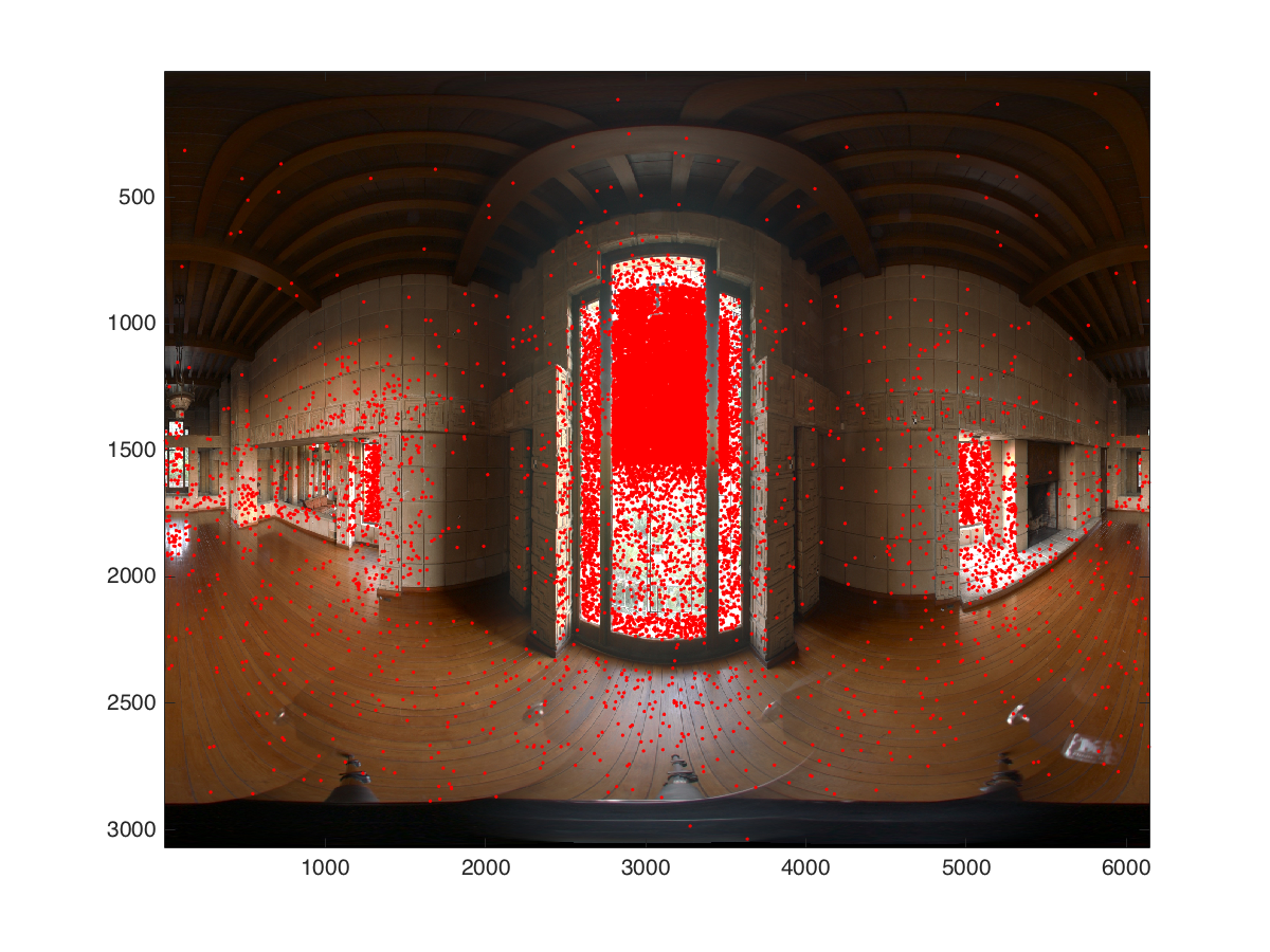
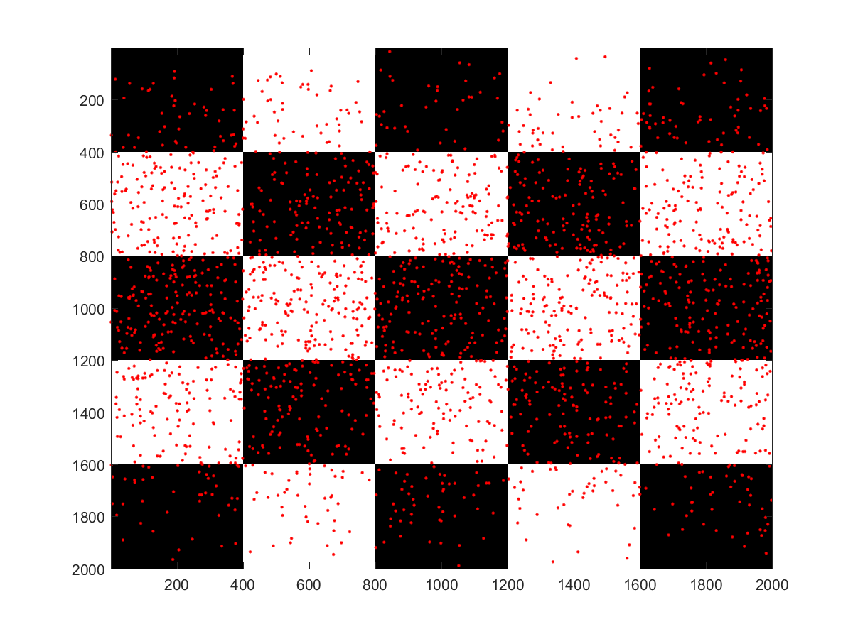
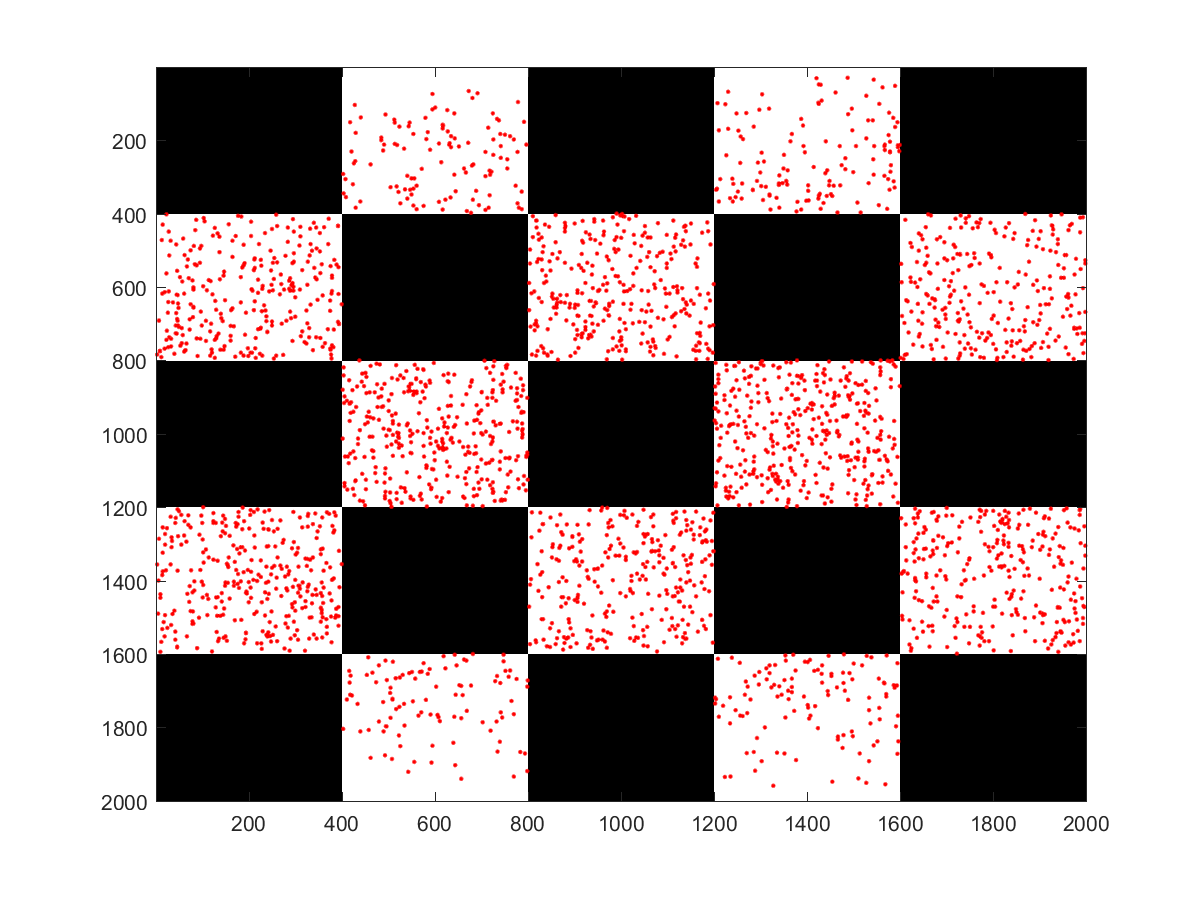
Validation

In order to validate my implementation I added a dumping mechanism which allows to progressively write all the sampled pixel coordinates of the environment map to a file. I wrote a small Matlab script to visualize the output. Below we can clearly observe the effect of the importance sampling. Both test cases use the luminance to create a scalar version of the image. In the first image the upper part of the center window is sampled more intensively compared to the lower part due to plants reducing the luminance in the lower half.

Homogenous participating media (20 Points)

In this last part I added global homogenous participating media to my scene. As I may wanted to add heterogenous media later (which ultimately I did not have the time for), I opted to implement ray marching.

Relevant files:

• media.h
• homogenous.cpp
• phasefunction.h
• isotropic.cpp
• greenstein.cpp
• schlick.cpp
• volume_direct_ems.cpp
• volume_path_mats.cpp

Ray-marching

Theory

In order to account for participating media, we have to solve the Volumetric Rendering Equation, which can be written as follows, neglecting radiance of the volume:

\( L(x,\vec{w})= T_r(x,x_z)L(x_z, \vec{w}) + \int_0^z T_r(x,x_t)\sigma_s(x_t)\int_{S^2} f_p(x_t,\vec{w}', \vec{w}) L_i(x_t, \vec{w}') d\vec{w}'dt \)

With

• \(\sigma_t\) is the extinction coefficient (controlled by the sum of simga_a (absorption) and sigma_s in the implementation)
• \(\sigma_s\) is the scattering coefficient (controlled by sigma_s)
• \(T_r(x,x_z)\) represents the transmittance from \(x\) to \(x_z\) which is given by \(e^{-\sigma_t||x-x_z||}\) in homogenous media.
• \(f_p(x_t,\vec{w}', \vec{w})\) is the media's associated phasefunction, which controls the scattering.

Below we can see some results obtained from the direct illumination integrator VolumeDirectEms defined in volume_direct_ems.cpp using 512 and 256 samples per pixel, respectively. The first image is using an isotropic phase function an the second one an anistropic backward scattering (Henyey-Greenstein).

Implementation details

The medium is defined by a handful of coefficients \((\sigma_t, \sigma_s)\) and registered in the scene. The Medium interface contains functions for calculating the transmittance and in-scattering (transmittance and inScattering, respectivly). Implementation of the Medium have to provide those functions as for example HomogenousMedium in homogenous.cpp does. The ray marching algorithm is implemented as described in the course notes and uses only single scattering! One more important note: It is crucial to randomly shift the initial position with rand()*dt, otherwise we have ugly-looking artifacts as shown below.

Phasefunctions

The Phasefunction describes the distribution of the scattered light. The interface of the Phasefunction is very similar to the one of BSDF. I've implemented the following phase functions:

Isotropic

Completly uniform scattering, can be associated with a diffuse BRDF.

\(f_p(\vec{w}',\vec{w}) = \frac{1}{4\pi}\)

Henyey-Greenstein (HG)

The Henyey-Greenstein function can be used to describe anisotropic scattering. Given a parameter \(g\) which represents the mean cosine between \(-\vec{w}\) and \(\vec{w}'\):

\(f_{pHG}(\theta) = \frac{1}{4\pi}\frac{1-g^2}{(1+g^2-2g\cos\theta)^{3/2}}\)

\(\theta = -\vec{w} \cdot \vec{w}'\)

If \(g = 0\) we recover isotropic scattering, \(g \lt 0\) will result in backward scattering and \(g \gt 0\) is forward scattering. Below we can see the effect of the parameter \(g\). We observe that the backward scattering is much brighter in the top part (closer to the light) compared to the forward scattering.

Schlick

There exits an approximation of the Henyey-Greenstein phase function, called Schlick approximation:

\(f_{pSchlick}(\theta) = \frac{1}{4\pi}\frac{1-k^2}{(1-k\cos\theta)^2}\)

\(\theta = -\vec{w} \cdot \vec{w}'\)

\(k = 1.55g - 0.55g^3\)

By simple observation, lacking the expensive pow operation, this should increase performance. The below images (Direct illumination 16 samples per pixel) have been rendered with Schlick (170s) and Greenstein (182s). While there is barely any visual difference the increase in speed seems to be worth it.

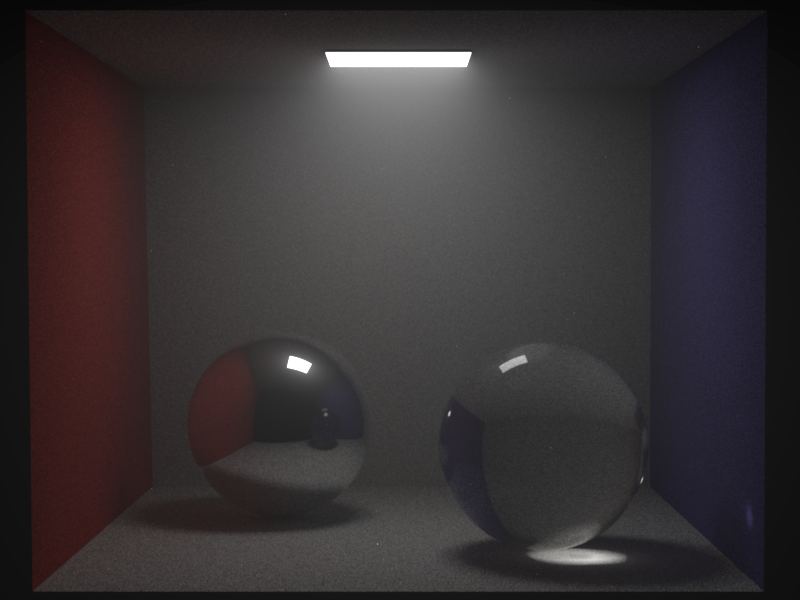
Global Illumination

Volumetric path tracing

In order to be able to render global illumination I extended the material path tracing integrator (PathMats) to account for participating media (volume_path_mats.cpp). The idea is pretty much the same as with VolumeDirectEMS. For each ray we perform a ray marching to account for single in-scattering. The sampled albedo of the BRDF will be reduced according to the transmittance of the media. The image below shows the Cornell box with a dielectric and mirrored sphere to showcase the global illumination.

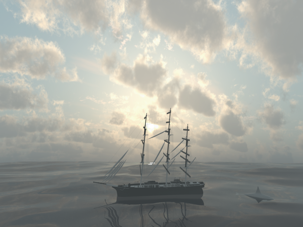
Final scene

The water is rendered with a two layered BRDF: the top layer is dielectric wave mesh with a scattering coefficient of water intIOR=1.33 and air extIOR=1.000277 while the lower layer is plain mesh with a microfacet (alpha=0.1) BRDF. The whole scene is covered in a homogenous participating media (sigma_a = sigma_s = 0.1, g=-0.5, stepsize = 0.1) which should represent fog over the water. The volumetric rendering equation is integrated using the VolumePathMats integrator which performs ray-marching with single scattering. The background of the scene is modeled with a matching environment map and slightly blurred with a depth of field camera. The image was generated using 2048 samples per pixel.

References

[1] Matt Pharr, Greg Humphreys. Monte Carlo Rendering with Natural Illumination. SIGGRAPH 2004

Resources

Environment maps: The Environment maps were obtained from USC.

Stanford dragon: The Stanford 3D Scanning Repository.

Normal/Texture maps: Normal and texture maps are from http://opengameart.org/.

Meshes: The meshes were obtained from http://tf3dm.com/.

The sky map is obtained from www.foro3d.com.